零均值归一化 ZNCC Zero normalized cross correlation
ZNCC: Zero normalized cross correlation, 零均值归一化是一种模板匹配中常用的互相关计算方法。它可以用于比较两个同维向量、窗口或样本之间的相关性。
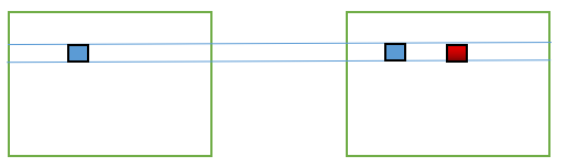
用于立体匹配的方法为:沿极线搜索左右目零均值归一化系数最小的两点,其坐标差即为视差。
立体匹配与深度计算
非基于深度学习的双目匹配算法大致分为四步:
- 采集图像
- 极线矫正
- 特征匹配
- 深度恢复
NCC 与 ZNCC 是衡量特征匹配的算法,一般采用 WTA 的方法得到视差。
双目视觉的几何原理并不是本文的重点,挖个坑以后再填
标准差、方差、协方差、相关系数
标准差
标准差描述了变量在整体变化过程中偏离均值的幅度。
\[\sigma = \sqrt{\frac{1}{n}\sum_{i=1}^{n}(X_i-\overline{X})^{2}}\]标准差越小,说明数据越集中。
所以在协方差中标准差作为分母对协方差进行了归一化。
方差
标准差的平方,衡量离散程度,计算每一个变量(观察值)与总体均数之间的差异。
\[Var(X)=\frac{1}{n}\sum_{i=1}^{n}(X_i-\overline{X})^{2}\]协方差
协方差反映两个随机变量相关程度,若两变量变化趋势相同,协方差为正值,反之为负。
\[Cov(X,Y)=E[(X-\overline{X})(Y-\overline{Y})]=E[XY]-E(X)E(Y)=\frac{1}{n-1}\sum_{i=1}^{n}(X_i-\overline{X})(Y_i-\overline{Y})\]相关系数
相关系数,亦称作皮尔逊相关系数。
相关系数是协方差的归一化(normalization), 消除了两个变量量纲/变化幅度不同的影响,单纯反映两个变量在每单位变化的相似程度。
\[p=\frac{Cov(X,Y)}{\sigma_{x}\sigma_{y}}\]或
\[r(X,Y)=\frac{Cov(X,Y)}{\sqrt{Var(X)Var(Y)} }\]其中:
- $X$ 是左图;
- $Y$ 是右图;
- $Cov(X,Y)$ 是左右两图的协方差;
- $Var(X)$ 是左图自己的方差;
NCC
简介
归一化相关性(normalization cross-correlation, NCC)使用类似于卷积核的n*n的匹配窗口对左右图像进行处理 ,检测左右匹配窗口的相似度,NCC 为左右图方框对应的 NCC 平均值。
双目匹配需要基线矫正,保证两幅图像只是在水平方向发生位移,产生视差。
公式
\[NCC(p,d)=\frac{\sum_{(x,y)\in W_p}^{}I_1(x,y)\cdot I_2(x+d,y) }{\sqrt{\sum_{(x,y)\in W_p}^{}I_1(x,y)^{2} \cdot \sum_{(x,y)\in W_p}^{}I_2(x,y)^{2}} }\]其中:
$NCC \in [-1,1]$,若$NCC=-1$,表示完全不相关;若 $NCC=1$,表示完全匹配
- $I_1$是左图,$I_2$是右图;
- $W_p$是以待匹配像素坐标为中心的匹配窗口;
- $I_1(x,y)$是左图中待匹配像素值,坐标$(p_x,p_y)$;
- $I_2(x+d,y)$是右图对应位置x坐标偏移d像素后的像素值,红框表示;
ZNCC
简介
零均值归一化(ZNCC, Zero-normalized cross-correlation), 相较 NCC 更鲁棒,因为 ZNCC 公式里减去了窗口内的均值,更能抵御光照的变化.
NCC 的公式记成 ZNCC 的公式,导致了很多误解。其实 NCC 的公式应用的特别少,多数使用的是 ZNCC 的公式,只不过有些人将 ZNCC 与 NCC 的名称弄混淆,导致 NCC 这个名词的知名度很高,其实多数使用的公式却是 ZNCC. [3]
公式
\[ZNCC(p,d)=\frac{\sum_{(x,y)\in W_p}^{}(I_1(x,y)-\overline{I_1}(p_x,p_y)\cdot (I_2(x,y)-\overline{I_2}(p_x+d,p_y) ) }{\sqrt{\sum_{(x,y)\in W_p}^{}(I_1(x,y)-\overline{I_1}(p_x,p_y))^{2} \cdot \sum_{(x,y)\in W_p}^{}(I_2(x,y)-\overline{I_2}(p_x+d,p_y))^{2}} }\]其中:
- $I_1$是左图,$I_2$是右图;
- $W_p$是以待匹配像素坐标为中心的匹配窗口;
- $I_1(x,y)$是左图中待匹配像素值,坐标$(p_x,p_y)$;
- $I_2(x+d,y)$是右图对应位置x坐标偏移d像素后的像素值,红框表示;
- $\overline{I}_1(p_x,p_y)$是左图匹配窗口所有像素均值;
- $\overline{I}_2(p_x+d,p_y)$是右图匹配所有窗口像素均值;
NCC与ZNCC的关系与向量理解[4]
更优雅的公式
NCC
NCC与ZNCC的唯一区别是不减去匹配窗口的均值亮度。
\[\frac{1}{n}\sum_{x,y}^{}\frac{1}{\sigma_f\sigma_t}f(x,y)t(x,y)\]ZNCC
$t(x,y)$:模板图像 待检测的图像,可以简单理解为右图,检测过程为在右图中寻找与子图像:$f(x,y)$的互相关被称为ZNCC,公式如下所示:
其中:
- $n$ is the number of pixels in $t(x,y)$ and $f(x,y)$
- $\sigma_f$ and $\sigma_t$ are the standard deviations of $f(x,y)$ and $t(x,y)$
- $\mu_f$ and $\mu_t$ are the average of $f(x,y)$ and $t(x,y)$
以向量的角度
在泛函分析中,ZNCC可以被看作是两个归一化向量的内积(dot product)
That is, if
$F(x,y)=f(x,y)-\mu_f$
and
$T(x,y)=t(x,y)-\mu_t$
then the ZNCC is the normalized dot product of the two vectors:
$\left \langle \frac{F}{\left | F \right | },\frac{T}{\left | T \right | } \right \rangle$
因此,如果$f$和$t$是实矩阵,那么ZNCC相当于$F$与$T$所对应的单位向量夹角的余弦值,两向量之间的交角为0即余弦值为1时即两向量方向相同,反之相反
It is also the 2-dimensional version of Pearson product-moment correlation coefficient.
where:
- $\left | \cdot \right |$ is the $L^2$norm.
- $\left \langle \cdot,\cdot \right \rangle $ is the inner product.
- Cauchy-Schwarz implies that the ZNCC has a range of $[-1,1]$.
$L^2$ norm is the Euclidean norm, and is defined as the sum of the squares of the vector elements.
$\left | F \right |=\sqrt{\sum_{1}^{n}(f(x,y)-\mu_f)}$
$\left | F \right | \left | T \right | =n\sigma_f\sigma _t$
And cos is:
$\cos \theta=\frac{a \cdot b}{\left | a \right | \left | b \right |}$
Implementation
C++
代码包含ZNCC和SAD,SAD的代码借鉴于 https://zhuanlan.zhihu.com/p/165405979
1
2
3
4
5
6
7
8
9
10
11
12
13
14
15
16
17
18
19
20
21
22
23
24
25
26
27
28
29
30
31
32
33
34
35
36
37
38
39
40
41
42
43
44
45
46
47
48
49
50
51
52
53
54
55
56
57
58
59
60
61
62
63
64
65
66
67
68
69
70
71
72
73
74
75
76
77
78
79
80
81
82
83
84
85
86
87
88
89
90
91
92
93
94
95
96
97
98
99
100
101
102
103
104
105
106
107
108
109
110
111
112
113
114
115
116
117
118
119
120
121
122
123
124
125
126
127
128
129
130
131
132
133
134
135
136
137
138
139
140
141
142
143
144
145
146
147
148
149
150
151
152
153
154
155
156
157
158
159
160
#include"iostream"
#include"opencv2/opencv.hpp"
#include"iomanip"
#include"cmath"
using namespace std;
using namespace cv;
class SAD
{
	public:
	SAD() :winSize(7), DSR(30), threshold(10){}
	SAD(int _winSize, int _DSR, int _threshold) :winSize(_winSize), DSR(_DSR), threshold(_threshold){}
	Mat computerSAD(Mat &L, Mat &R); // 计算SAD
	Mat computerZNCC(Mat &L, Mat &R); //计算ZNCC

	private:
	int winSize; //卷积核的尺寸
	int DSR; //视差搜索范围
	int threshold;
};

Mat SAD::computerZNCC(Mat &L, Mat &R)
{
	int Height = L.rows;
	int Width = L.cols;

	Mat Kernel_L(Size(winSize, winSize), CV_8U, Scalar::all(0));
	Mat Kernel_R(Size(winSize, winSize), CV_8U, Scalar::all(0));

	Mat Disparity(Height, Width, CV_8U, Scalar(0)); //视差图
	for (int i = 0; i < Width - winSize; i++) {
		for (int j = 0; j < Height - winSize; j++) {
			Mat MM(1, DSR, CV_32F, Scalar(0));
			if(L.at<uchar>(j,i) > threshold)
			{
				Kernel_L = L(Rect(i, j, winSize, winSize));
				for (int k = 0; k < DSR; k++) {

					int x = i - k;
					if (x <= Width - winSize && x >=0) {
						Kernel_R = R(Rect(x, j, winSize, winSize));

						Scalar mean_L = mean(Kernel_L);
						Scalar mean_R = mean(Kernel_R);

						int64_t  sum_upper = 0;
						int64_t  square_sum_L = 0;
						int64_t  square_sum_R = 0;
						for (int a = j; a < j + winSize; a++) {
							for (int b = i; b < i + winSize; b++) {
								sum_upper += (L.at<char>(a, b) - mean_L[0]) * ((R.at<char>(a, b-k) - mean_R[0]));
								square_sum_L += (L.at<char>(a, b) - mean_L[0]) * ((L.at<char>(a, b) - mean_L[0]));
								square_sum_R += (R.at<char>(a, b-k) - mean_R[0]) * ((R.at<char>(a, b-k) - mean_R[0]));
							}
						}

						// cout << "Kernel_L" << endl
						// 	 << Kernel_L << endl;
						// cout << "Kernel_R:" << endl
						// 	 << Kernel_R << endl;
						// cout << "mean_L:" << mean_L[0] << endl;
						// cout << "mean_R:" << mean_R[0] << endl;
						// cout << "sum_upper:" << sum_upper << endl;
						// cout << "square_sum_L:" << square_sum_L << endl;
						// cout << "square_sum_R:" << square_sum_R << endl;
						// cout << "sqrt:" << (sqrt(square_sum_L) * sqrt(square_sum_R)) << endl;
						// cout << "MM:" << sum_upper / (sqrt(square_sum_L) * sqrt(square_sum_R)) << endl;

						if(sqrt(square_sum_L * square_sum_R) != 0) {
							MM.at<float>(k) = sum_upper / (sqrt(square_sum_L) * sqrt(square_sum_R));
						}
						// cout<<"MM full:"<<MM<<endl;
						// cout<<MM.at<float>(k)<<endl;
					}
				}
			}
			Point maxLoc;
			minMaxLoc(MM, NULL, NULL, NULL, &maxLoc);
			int loc = maxLoc.x;
			// cout<<"loc:"<<loc<<endl;
			// cout<<loc<<endl;
			// loc = DSR-loc;
			// Disparity.at<char>(j, i) = loc * 16;
			// cout << "Disparity:" << endl<< Disparity << endl;
			Disparity.at<char>(j, i) = loc;
		}
		// double rate = double(i) / (Width);
		// cout << "已完成" << setprecision(2) << rate * 100 << "%" << endl; //显示处理进度
	}
	// cout<<"Disparity:"<<endl<<Disparity<<endl;
	return Disparity;
}

Mat SAD::computerSAD(Mat &L, Mat &R)
{
	int Height = L.rows;
	int Width = L.cols;
	Mat Kernel_L(Size(winSize, winSize), CV_8U, Scalar::all(0));
	Mat Kernel_R(Size(winSize, winSize), CV_8U, Scalar::all(0));
	Mat Disparity(Height, Width, CV_8U, Scalar(0)); //视差图

	for (int i = 0; i < Width - winSize; i++) //左图从DSR开始遍历
	{
		for (int j = 0; j<Height - winSize; j++){
			if(L.at<uchar>(j,i) > threshold)
			{
				Kernel_L = L(Rect(i, j, winSize, winSize));
				Mat MM(1, DSR, CV_32F, Scalar(0));
				for (int k = 0; k<DSR; k++)
				{
					int x = i - k;
					if (x >= 0)
					{
						Kernel_R = R(Rect(x, j, winSize, winSize));
						Mat Dif;
						absdiff(Kernel_L, Kernel_R, Dif); // 求差的绝对值之和
						Scalar ADD = sum(Dif);
						float a = ADD[0];
						MM.at<float>(k) = a;
					}
				}
				Point minLoc;
				minMaxLoc(MM, NULL, NULL, &minLoc, NULL);
				int loc = minLoc.x;
				// int loc=DSR-loc;
				// Disparity.at<char>(j, i) = loc * 16;
				Disparity.at<char>(j, i) = loc;
			}
		}

		// double rate = double(i) / (Width);
		// cout << "已完成" << setprecision(2) << rate * 100 << "%" << endl; // 显示处理进度
	}
	return Disparity;
}

int main(int argc, char* argv[])
{
	Mat Img_L = imread("im2.png", 0);
	Mat Img_R = imread("im6.png", 0);
	// Mat Img_L = imread("m_denoise_l.png", 0);
	// Mat Img_R = imread("m_denoise_r.png", 0);
	Mat Disparity; //创建视差图

	SAD myZNCC(7, 40, 1); //参数 winSize DSR threshold
	SAD mySAD(7, 30, 10);

	Disparity = myZNCC.computerZNCC(Img_L, Img_R);
	// Disparity = mySAD.computerSAD(Img_L, Img_R);


	// imshow("Teddy_L", Img_L);
	// imshow("Teddy_R", Img_R);
	imshow("Disparity", Disparity); //显示视差图
	waitKey();
	imwrite("Disparity.png", Disparity);
	// system("pause");  //按任意键退出
	return 0;
}
Python
边缘像素如何处理?
为了简化计算,这里并没有对图像进行裁切边缘的操作。 scipy.ndimage.uniform_filter 函数是一个多维均匀滤波器,滤波器窗口大小为 size 参数指定,默认为3. 使用改函数进行匹配窗口的平均值计算,该函数的 mode 参数可以设置边缘情况的处理方式。
scipy.ndimage.uniform_filter(input, size=3, output=None, mode='reflect', cval=0.0, origin=0, *, axes=None)
The mode parameter determines how the input array is extended when the filter overlaps a border. By passing a sequence of modes with length equal to the number of dimensions of the input array, different modes can be specified along each axis. Default value is ‘reflect’. The valid values and their behavior is as follows:
- ‘reflect’ (d c b a |a b c d | d c b a) The input is extended by reflecting about the edge of the last pixel. This mode is also sometimes referred to as half-sample symmetric.
- ‘constant’ (k k k k |a b c d| k k k k) The input is extended by filling all values beyond the edge with the same constant value, defined by the cval parameter.
- ‘nearest’ (a a a a | a b c d| d d d d) The input is extended by replicating the last pixel.
NCC
1
2
3
4
5
6
7
8
9
10
11
12
13
14
15
16
17
18
19
20
21
22
23
24
25
26
27
28
29
30
31
32
33
34
35
36
37
38
39
40
41
42
43
44
45
46
47
48
49
50
51
52
53
54
55
56
57
58
59
60
61
62
from PIL import Image
from pylab import *
import cv2
from numpy import *
from numpy.ma import array
from scipy.ndimage import filters
import scipy.misc
import imageio


def plane_sweep_ncc(im_l, im_r, start, steps, wid):
    """ 使用归一化的互相关计算视差图像 """
    m, n = im_l.shape
    # 创建保存不同求和值的数组
    mean_l = zeros((m, n))
    mean_r = zeros((m, n))
    s = zeros((m, n))
    s_l = zeros((m, n))
    s_r = zeros((m, n))
    # 创建保存深度平面的数组
    dmaps = zeros((m, n, steps))

    # # only for ZNCC
    # # 计算图像块的平均值
    # filters.uniform_filter(im_l, wid, mean_l)
    # filters.uniform_filter(im_r, wid, mean_r)
    # # 归一化图像
    # norm_l = im_l - mean_l
    # norm_r = im_r - mean_r

    # 尝试不同的视差
    #  steps 是视差的最大可能值
    for displ in range(steps):
        # 将左边图像移动到右边,计算加和
        # np.roll() 函数将数组元素向后移动 -displ - start 个单位
        # 和归一化, s 为 ncc 的分子
        filters.uniform_filter(np.roll(norm_l, -displ - start) * norm_r, wid, s)

        filters.uniform_filter(np.roll(norm_l, -displ - start) * np.roll(norm_l, -displ - start), wid, s_l)
        filters.uniform_filter(norm_r * norm_r, wid, s_r)  # 和反归一化
        # 保存 ncc 的值在 dmaps 中
        dmaps[:, :, displ] = s / sqrt(s_l * s_r)
        # 为每个像素选取最佳深度
        # 选取最大的的 dmaps ,即视差,WTA
    return np.argmax(dmaps, axis=2)

# img is size: 1800 x 1500
im_l = array(Image.open(r'D:/Dataset/teddyF/im2.ppm').convert('L'), 'f')
im_r = array(Image.open(r'D:/Dataset/teddyF/im6.ppm').convert('L'), 'f')

# 参数:与图像尺寸有关,需要根据图像尺寸调整
# 视差的最大值
steps = 180
# 匹配窗口起始偏置,一般为0,因为视差不可能为负
start = 0
# 匹配窗口的宽度
wid = 20

res = plane_sweep_ncc(im_l, im_r, start, steps, wid)
imshow(res)
show()
ZNCC
Pixelwise ZNCC, 适用于处理事件帧。
1
2
3
4
5
6
7
8
9
10
11
12
13
14
15
16
17
18
19
20
21
22
23
24
25
26
27
28
29
30
31
32
33
34
35
36
37
38
39
40
41
42
43
44
45
46
47
48
49
import cv2
import numpy as np

class SAD:
	def __init__(self, winSize=7, DSR=30, threshold=10):
		self.winSize = winSize
		self.DSR = DSR
		self.threshold = threshold

	def computerZNCC(self, L, R):
		Height, Width = L.shape
		Kernel_L = np.zeros((self.winSize, self.winSize), dtype=np.uint8)
		Kernel_R = np.zeros((self.winSize, self.winSize), dtype=np.uint8)
		Disparity = np.zeros((Height, Width), dtype=np.uint8)
		for i in range(Width - self.winSize):
			for j in range(Height - self.winSize):
				MM = np.zeros((1, self.DSR), dtype=np.float32)
				if L[j, i] > self.threshold:
					Kernel_L = L[j:j+self.winSize, i:i+self.winSize]
					for k in range(self.DSR):
						x = i - k
						if x <= Width - self.winSize and x >= 0:
							Kernel_R = R[j:j+self.winSize, x:x+self.winSize]
							mean_L = np.mean(Kernel_L)
							mean_R = np.mean(Kernel_R)
							sum_upper = 0
							square_sum_L = 0
							square_sum_R = 0
							for a in range(j, j+self.winSize):
								for b in range(i, i+self.winSize):
									sum_upper += (L[a, b] - mean_L) * (R[a, b-k] - mean_R)
									square_sum_L += (L[a, b] - mean_L) ** 2
									square_sum_R += (R[a, b-k] - mean_R) ** 2
							if np.sqrt(square_sum_L * square_sum_R) != 0:
								MM[0, k] = sum_upper / np.sqrt(square_sum_L * square_sum_R)
							min_val,max_val,min_indx,max_indx = cv2.minMaxLoc(MM)
							loc = np.where(MM == max_val)
							Disparity[j, i] = loc[1][0]
		return Disparity


if __name__ == '__main__':
	Img_L = cv2.imread("m_denoise_l.png", 0)
	Img_R = cv2.imread("m_denoise_r.png", 0)
	myZNCC = SAD(7, 40, 130)
	Disparity = myZNCC.computerZNCC(Img_L, Img_R)
	# cv2.imshow("Disparity", Disparity)
	# cv2.waitKey()
	cv2.imwrite("Disparity.png", Disparity)
1
2
3
4
5
6
7
8
9
10
11
12
13
14
15
16
17
18
19
20
21
22
23
24
25
26
27
28
29
30
31
32
33
34
35
36
37
38
39
40
41
42
43
44
45
46
47
48
49
50
51
52
53
54
55
56
57
58
59

from PIL import Image
from pylab import *
import cv2
from numpy import *
from numpy.ma import array
from scipy.ndimage import filters
import scipy.misc
import imageio


def plane_sweep_ncc(im_l, im_r, start, steps, wid):
    """ 使用归一化的互相关计算视差图像 """
    m, n = im_l.shape
    # 创建保存不同求和值的数组
    mean_l = zeros((m, n))
    mean_r = zeros((m, n))
    s = zeros((m, n))
    s_l = zeros((m, n))
    s_r = zeros((m, n))
    # 创建保存深度平面的数组
    dmaps = zeros((m, n, steps))
    # 计算图像块的平均值
    filters.uniform_filter(im_l, wid, mean_l)
    filters.uniform_filter(im_r, wid, mean_r)
    # 归一化图像
    norm_l = im_l - mean_l
    norm_r = im_r - mean_r
    # 尝试不同的视差
    #  steps 是视差的最大可能值
    for displ in range(steps):
        # 将左边图像移动到右边,计算加和
        # np.roll() 函数将数组元素向后移动 -displ - start 个单位
        # 和归一化, s 为 ncc 的分子
        filters.uniform_filter(np.roll(norm_l, -displ - start) * norm_r, wid, s)

        filters.uniform_filter(np.roll(norm_l, -displ - start) * np.roll(norm_l, -displ - start), wid, s_l)
        filters.uniform_filter(norm_r * norm_r, wid, s_r)  # 和反归一化
        # 保存 ncc 的值在 dmaps 中
        dmaps[:, :, displ] = s / sqrt(s_l * s_r)
        # 为每个像素选取最佳深度
        # 选取最大的的 dmaps ,即视差,WTA
    return np.argmax(dmaps, axis=2)

# img is size: 1800 x 1500
im_l = array(Image.open(r'D:/Dataset/teddyF/im2.ppm').convert('L'), 'f')
im_r = array(Image.open(r'D:/Dataset/teddyF/im6.ppm').convert('L'), 'f')

# ZNCC参数:与图像尺寸有关,需要根据图像尺寸调整
# 视差的最大值
steps = 180
# 匹配窗口起始偏置,一般为0,因为视差不可能为负
start = 0
# 匹配窗口的宽度
wid = 20

res = plane_sweep_ncc(im_l, im_r, start, steps, wid)
imshow(res)
show()
Result and groundtruth
Datasets
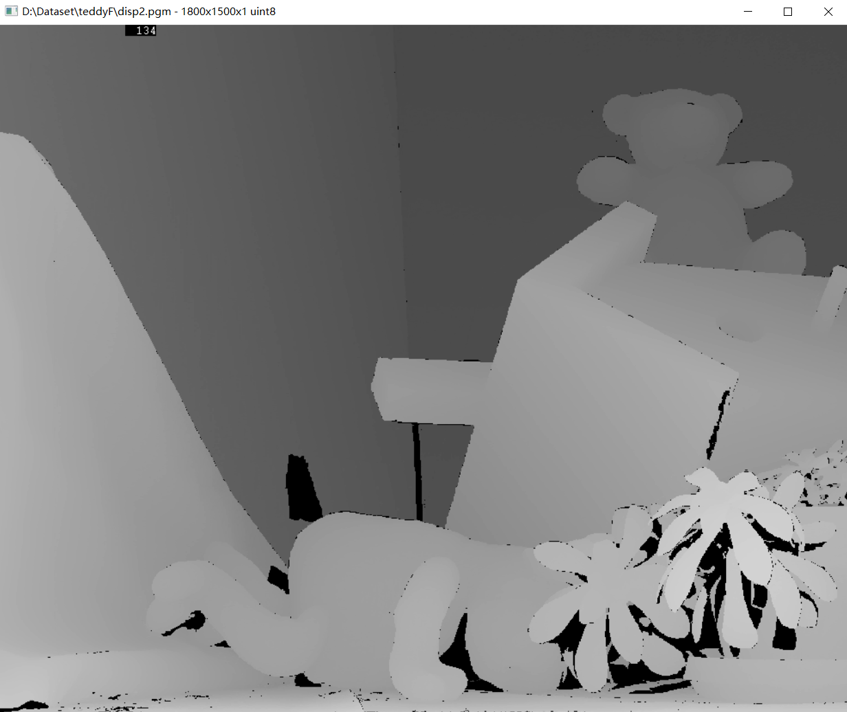
Middleburry 2003 Stereo datasets with ground truth 使用teddyF/im2.ppm和teddyF/im6.ppm作为测试图像。
Output result
Python
匹配窗口宽度25, 视差图中存在缺陷,需要后续处理,初步验证了NCC和ZNCC算法的正确性。
右边缘由于没有进行裁切,所以边缘的视差值不准确 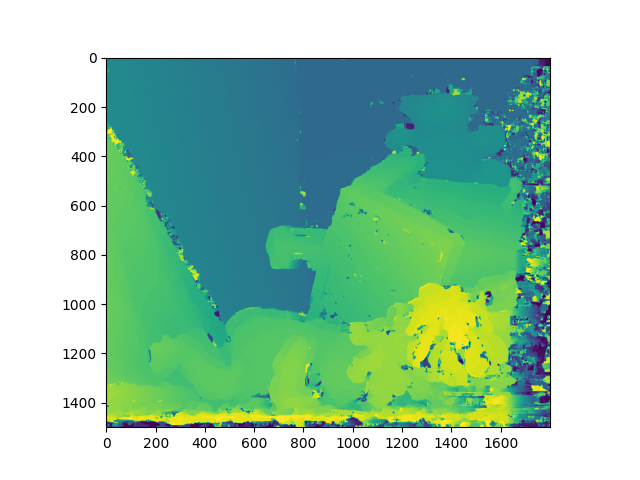
Ground truth
Reference
[4]Cross-correlation_Wikipedia